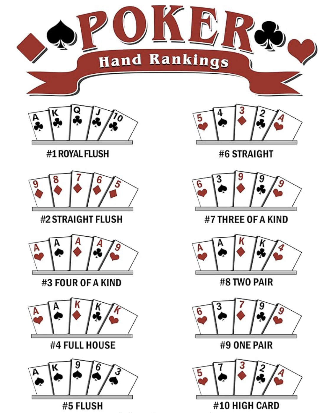
Example 4.1 Texas hold’em is one of the most popular variant of the card game of poker. Essentially, the players in the game bet on the rankings of their hand of five cards (illustrated in the figure below). For the game to be fair, a hand of higher values must have lower probability than a hand of lower values. Compute the probability for each type of hand.
Solution. To apply Definition 3.1, we first determine the total number of possible five-card hands from a standard 52-card deck. The total number of combinations is: \[\binom{52}{5} = \frac{52 \times 51 \times 50 \times 49 \times 48}{5 \times 4 \times 3 \times 2 \times 1} = 2,598,960\]
We then find the number of combinations for each hand type. As an illustration, we only compute the case of Full House.
A full house consists of three cards of one rank and two cards of another rank. The number of ways to choose the rank for the triplet is \(\binom{13}{1} = 13\) , and the number of ways to choose 3 cards of that rank is \(\binom{4}{3} = 4\) . The number of ways to choose the rank for the pair is \(\binom{12}{1} = 12\) , and the number of ways to choose 2 cards of that rank is \(\binom{4}{2} = 6\) . Therefore, the total number of full houses is: \(\binom{13}{1}\binom{4}{3}\cdot\binom{12}{1}\binom{4}{2} = 3,744\).
Thus, the probability is: \[P(\text{Full House}) = \frac{3,744}{2,598,960} \approx 0.144\%\]
Example 4.2 (Newton-Pepys problem) The Newton-Pepys problem is a classical probability problem involving dice rolls, posed in correspondence between Samuel Pepys, a famous diarist and government official, and Isaac Newton in 1693. The problem concerns which of the following three events is most likely when rolling fair dice:
At least one 6 appears when 6 fair dice are rolled.
At least two 6’s appear when 12 fair dice are rolled.
At least three 6’s appear when 18 fair dice are rolled.
Solution. We compute the probabilities for each scenario:
Probability of at least one 6 in six rolls of a single die:
The probability of not rolling a 6 in six rolls is: \[P(\text{no 6 in six rolls}) = \frac{5^6}{6^6}\] Thus, the probability of at least one 6 in six rolls is: \[P(\text{at least one 6}) = 1 - \frac{5^6}{6^6} \approx 0.67\]
Probability of at least two 6s in twelve rolls of a single die:
We use the complement, finding the probabilities of getting 0 or 1 six. The probability of getting exactly 0 sixes in twelve rolls is similar as above. The probability of getting exactly 1 six is: \[P(1 \text{ six}) = \binom{12}{1} \frac{5^{11}}{6^{12}}\] Thus, the probability of at least two 6s is: \[P(\text{at least two 6s}) = 1 - P(0 \text{ six})-P(1 \text{ six}) \approx 0.62\]
Probability of at least three 6s in eighteen rolls of a single die:
Similarly, we calculate the complement, finding the probabilities of getting fewer than 3 sixes. \[\begin{aligned}
P(\text{at least three 6s}) &= 1 - P(0\text{ six}) -P(1\text{ six}) - P(2\text{ sixes}) \\ \\
&= 1- \frac{5^{18} + \binom{18}{1}5^{17} + \binom{18}{2} 5^{16}}{6^{18}} \approx 0.60
\end{aligned}
\]
Thus, \(P(\text{one 6 in 6 rolls}) > P(\text{two 6s in 12 rolls}) > P(\text{three 6s in 18 rolls})\).
Intuitively, this is because as the number of dice increases, the likelihood of matching higher thresholds does not keep pace with the probability of rolling individual sixes. This is perhaps contrary to most people’s common sense: the more dice rolled, the more likely to see the sixes.
# generate a deck of cardsdeck.grid <-expand.grid(c(1:10,'J','Q','K','A'), c('♠','♥','♦','♣'))# convert the grid to a vectordeck <-do.call(paste0, deck.grid)# total number of simulationsN <-100000# number of target handK <-0# for random generatorset.seed(1000)for (j in1:N) {# a random five-cards hand hand <-sample(deck, 5)# drop the color num <-substr(hand, 1, nchar(hand)-1)# Full House have only two distinguished numbersif ( length(unique(num)) ==2 ) { K <- K +1 }}# compute the probabilityP <- K / Nsprintf("Prob of Full House: %.3f %%", P*100)