38 Covariance
For more than one random variable, it is also of interest to know the relationship between them. Are they dependent? How strong is the dependence? Covariance and correlation are intended to measure that dependence. But they only capture a particular type of dependence, namely linear dependence.
Definition 38.1 (Covariance) The covariance between random variables \(X\) and \(Y\) is defined as \[Cov(X,Y)=E[(X-EX)(Y-EY)].\]
The covariance between \(X\) and \(Y\) reflects how much \(X\) and \(Y\) simultaneously deviate from their respective means.
Theorem 38.1 For any random variables \(X\) and \(Y\), \[Cov(X,Y)=E(XY)-E(X)E(Y).\]
Proof. Let \(\mu_{X}=E(X)\) and \(\mu_{Y}=E(Y)\). By definition, \[\begin{aligned} Cov(X,Y) & =E(XY-\mu_{X}Y-\mu_{Y}X+\mu_{X}\mu_{Y})\\ & =E(XY)-\mu_{X}E(Y)-\mu_{Y}E(X)+\mu_{X}\mu_{Y}\\ & =E(XY)-E(X)E(Y).\end{aligned}\]
Theorem 38.2 If \(X,Y\) are independent, they are uncorrelated. But the converse is false.
Proof.
- \(Cov(X,Y)=E(XY)-E(X)E(Y)\). Independence implies \(E(XY)=E(X)E(Y)\). Thus, \(Cov(X,Y)=0\).
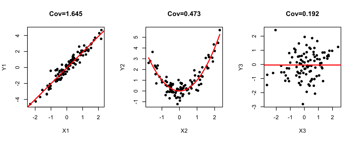
- \(Cov(X,Y)=0\) does not necessarily imply independence. Consider the following counter example. Let \(X\) be a random variable that takes three values -1, 0, 1 with equal probability. And \(Y=X^{2}\). \(X\) and \(Y\) are clearly dependent. But they their covariance is 0. Since \(E(X)=0\), \(E(Y)=2/3\), \(E(XY)=E(X^{3})=0\), \(Cov(X,Y)=0\).
Linear dependency
Covariance and correlation provide measures of the extend to which two random variables are linearly related. It is possible that the covariance is \(0\) even when \(X\) and \(Y\) are dependent but the relationship is nonlinear.
Proposition 38.1 Covariance has the following properties:
- \(Cov(X,X)=Var(X)\)
- \(Cov(X,Y)=Cov(Y,X)\)
- \(Cov(cX,Y)=Cov(X,cY)=c\left[Cov(X,Y)\right]\)
- \(Cov(X+Y,Z)=Cov(X,Z)+Cov(Y,Z)\)
- \(Var(X+Y)=Var(X)+Var(Y)+2Cov(X,Y)\)
Proof. We only prove the variance-covariance property: \[\begin{aligned} Var(X+Y) & =E[(X+Y-\mu_{X}-\mu_{Y})^{2}]\\ & =E[(X-\mu_{X})^{2}+(Y-\mu_{Y})^{2}+2(X-\mu_{X})(Y-\mu_{Y})]\\ & =Var(X)+Var(Y)+2Cov(X,Y).\end{aligned}\]
Theorem 38.3 For random variables \(X_1,X_2,\dots,X_n\), it holds that \[Var\left(\sum_{i=1}^{n}X_{i}\right)=\sum_{i=1}^{n}Var(X_{i})+ 2\sum_{i<j}Cov(X_{i},X_{j}).\]
If \(X_1,X_2,\dots,X_n\) are identically distributed and have the same covariance relationships (symmetric), then \[Var\left(\sum_{i=1}^{n}X_{i}\right)=nVar(X_1)+2\binom{n}{2}Cov(X_1,X_2).\]
While \(\text{Cov}(X,Y)\) quantifies how \(X\) and \(Y\) vary together, its magnitude also depends on the absolute scales of \(X\) and \(Y\) (multiply \(X\) by a constant \(c\), the covariance will be different). To establish a measure of association between \(X\) and \(Y\) that is unaffected by arbitrary changes in the scales of either variable, we introduce a “standardized covariance” called correlation.
Definition 38.2 (Correlation) The correlation between random variables \(X\) and \(Y\) is defined as \[Corr(X,Y)=\frac{Cov(X,Y)}{\sqrt{Var(X)Var(Y)}}.\]
By convention, we denote correlation by Greek letter \(\rho\equiv Corr(X,Y)\).
Unlike covariance, scaling \(X\) or \(Y\) has no effect on the correlation. We can verify this: \[Corr(cX,Y)=\frac{Cov(cX,Y)}{\sqrt{Var(cX)Var(Y)}}=\frac{cCov(X,Y)}{c\sqrt{Var(X)Var(Y)}}=Corr(X,Y).\]
Theorem 38.4 For any random variable \(X\) and \(Y\), \[-1\leq Corr(X,Y)\leq1.\]
Proof. Without loss of generality, assume \(X,Y\) both have variance 1, since scaling does not change the correlation. Let \(\rho=Corr(X,Y)=Cov(X,Y)\). Then \[\begin{aligned} Var(X+Y) & =Var(X)+Var(Y)+2Cov(X,Y)=2+2\rho\geq0,\\ Var(X-Y) & =Var(X)+Var(Y)-2Cov(X,Y)=2-2\rho\ge0.\end{aligned}\] Thus \(-1\leq\rho\leq1\).
- \(X\) and \(Y\) are positively correlated if \(\rho_{XY}>0\);
- \(X\) and \(Y\) are negatively correlated if \(\rho_{XY}<0\);
- \(X\) and \(Y\) are uncorrelated if \(\rho_{XY}=0\).
Theorem 38.5 Suppose that \(X\) is a random variable and \(Y=aX+b\) for some constants \(a,b\), where \(a\neq0\). If \(a>0\), then \(\rho_{XY}=1\). If \(a<0\), then \(\rho_{XY}=-1\).
Proof. If \(Y=aX+b\), then \(E(Y)=aE(X)+b\). Thus, \(Y-E(Y)=a(X-E(X))\). Therefore, \[Cov(X,Y)=aE[(X-EX)^{2}]=aVar(X).\] Since \(Var(Y)=a^{2}Var(X)\), \(\rho_{XY}=\frac{a}{|a|}\). The theorem thus follows.
Correlation analysis
A correlation matrix shows the pairwise correlation coefficients between variables. It’s one of the most common tools for exploring relationships in multivariate data.
# variables for analysis
vars <- mtcars[, 1:4]

# compute the correlation matrix
print(cor(vars))
mpg cyl disp hp
mpg 1.000 -0.852 -0.848 -0.776
cyl -0.852 1.000 0.902 0.832
disp -0.848 0.902 1.000 0.791
hp -0.776 0.832 0.791 1.000Example 38.1 Let \(X\sim \text{HGeom}(w,b,n)\). Find \(Var(X)\).
Solution. Interpret \(X\) as the number of white balls in a sample of size \(n\) from an box with \(w\) white and \(b\) black balls. We can represent \(X\) as the sum of indicator variables, \(X=I_{1}+\cdots+I_{n}\) , where \(I_{j}\) is the indicator of the \(j\)-th ball in the sample being white. Each \(I_{j}\) has mean \(p=w/(w+b)\) and variance \(p(1-p)\), but because the \(I_{j}\) are dependent, we cannot simply add their variances. Instead, \[\begin{aligned} Var(X) & =Var\left(\sum_{j=1}^{n}I_{j}\right)\\ & =Var(I_{1})+\cdots+Var(I_{n})+2\sum_{i<j}Cov(I_{i},I_{j})\\ & =np(1-p)+2\binom{n}{2}Cov(I_{i},I_{j})\end{aligned}\]
In the last step, because of symmetry, for every pair \(i\) and \(j\), \(Cov(I_{i},I_{j})\) are the same. \[\begin{aligned} Cov(I_{i},I_{j}) & =E(I_{i}I_{j})-E(I_{i})E(I_{j})\\ & =P(i\textrm{ and }j\textrm{ both white})-P(i\textrm{ is white})P(j\textrm{ is white})\\ & =\frac{w}{w+b}\cdot\frac{w-1}{w+b-1}-p^{2}\\ & =p\frac{Np-1}{N-1}-p^{2}\\ & =\frac{p(p-1)}{N-1}\end{aligned}\]
where \(N=w+b\). Plugging this into the above formula and simplifying, we eventually obtain \[Var(X)=np(1-p)+n(n-1)\frac{p(p-1)}{N-1}=\frac{N-n}{N-1}np(1-p).\] This differs from the Binomial variance of \(np(1-p)\) by a factor of \(\frac{N-n}{N-1}\). This discrepancy arises because the Hypergeometric story involves sampling without replacement. As \(N\to\infty\), it becomes extremely unlikely that we would draw the same ball more than once, so sampling with or without replacement essentially become the same.