47  Normal distribution

The most widely used model for random variables with continuous distributions is the family of normal distributions. One reason is that many real world samples appears to be normally distributed (the mass centered around the mean). The other reason is because of the Central Limit Theorem (will be discussed in later chapters), which essentially says the sum (or mean) or any random samples are approximately normal.

Definition 47.1 (Standard Normal) A random variable \(Z\) has the standard Normal distribution with mean \(0\) and variance \(1\), denoted as \(Z\sim N(0,1)\), if \(Z\) has a PDF that follows \[f(z)=\frac{1}{\sqrt{2\pi}}e^{-z^{2}/2}.\]

This is a valid PDF because \(\int_{-\infty}^{\infty}f(z)dz=1\), which directly follows from the Gaussian integral. We further verify its mean and variance:

\[E(Z)=\int_{-\infty}^{+\infty}z\cdot\frac{1}{\sqrt{2\pi}}e^{-z^{2}/2}dz=0\quad\textrm{by symmetry.}\]

\[\begin{aligned} Var(Z) & =E(Z^{2})-(EZ)^{2}=E(Z^{2})\\ & =\int_{-\infty}^{+\infty}z^{2}\cdot\frac{1}{\sqrt{2\pi}}e^{-z^{2}/2}dz\\ & =\frac{2}{\sqrt{2\pi}}\int_{0}^{\infty}\underbrace{z}_{u}\cdot\underbrace{ze^{-z^{2}/2}dz}_{dv}\\ & =\frac{2}{\sqrt{2\pi}}\left\{ \left[z(-e^{-z^{2}/2})\right]_{0}^{\infty}+\underbrace{\int_{0}^{\infty}e^{-z^{2}/2}dz}_{\sqrt{2\pi}/2}\right\} \\ & =1.\end{aligned}\]

Definition 47.2 (The \(\Phi\) function) The CDF of standard normal distribution is usually denoted by \(\Phi\). Therefore, \[\Phi(z)=\frac{1}{\sqrt{2\pi}}\int_{-\infty}^{z}e^{-t^{2}/2}dt.\] By symmetry, we have \(\Phi(-z)=1-\Phi(z)\).

To find the value of \(\Phi(z)\), we need to use the normal probability table or statistical software.

Definition 47.3 (General Normal) Let \(X=\mu+\sigma Z\) where \(Z\sim N(0,1)\). Then we say \(X\) has the Normal distribution with mean \(\mu\) and variance \(\sigma^{2}\), denoted as \(X\sim N(\mu,\sigma^{2})\). The PDF of \(X\) is given by \[f(x)=\frac{1}{\sqrt{2\pi\sigma^{2}}}\exp\left[-\frac{1}{2}\left(\frac{x-\mu}{\sigma}\right)^{2}\right].\]

The mean and variance of \(X\) can be easily verified by the properties of expectation and variance. \[\begin{aligned} E(X) & =E(\mu+\sigma Z)=\mu+\sigma E(Z)=\mu,\\ Var(X) & =Var(\mu+\sigma Z)=\sigma^{2}Var(Z)=\sigma^{2}.\end{aligned}\]

To verify the PDF, we utilize the standard normal CDF: \[P(X\leq x)=P\left(\frac{X-\mu}{\sigma}\leq\frac{x-\mu}{\sigma}\right)=\Phi\left(\frac{x-\mu}{\sigma}\right)\]

The PDF is the derivative of the CDF, \[f(x)=\frac{1}{\sigma}\Phi'\left(\frac{x-\mu}{\sigma}\right)=\frac{1}{\sigma\sqrt{2\pi}}\exp\left[-\frac{1}{2}\left(\frac{x-\mu}{\sigma}\right)^{2}\right].\]

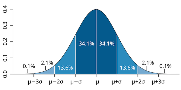
Proposition 47.1 (Three-sigma rule) The normal distribution has the following properties: \[\begin{aligned} P(|X-\mu|\leq\sigma) & \approx 0.68\\ P(|X-\mu|\leq2\sigma) & \approx 0.95\\ P(|X-\mu|\leq3\sigma) & \approx 0.997\\ \end{aligned}\] Critical values in standard normal: \(\Phi(-1)\approx0.16,\Phi(-2)\approx0.025,\Phi(-3)\approx0.0015\).

Theorem 47.1 (Standardization) Let \(X\) have the Normal distribution with mean \(\mu\) and variance \(\sigma^{2}\). Let \(F\) be the CDF of \(X\). Then the standardization of \(X\) \[Z=\frac{X-\mu}{\sigma}\] has the standard normal distribution, and, for all \(x\): \[F(x)=\Phi\left(\frac{x-\mu}{\sigma}\right).\]

Example 47.1 Suppose the test score of a class of 50 students is normally distributed with mean 80 and standard deviation 20 (the total mark is 100). A student has scored 90. What is his percentile in the class?

Solution. \(X\sim N(80,20)\). We want to find \(P(X<90)\). Standardize the distribution: \[P(X<90)=P\left(\frac{X-80}{20}<\frac{90-80}{20}\right)=\Phi(0.5)\approx0.69.\]

Theorem 47.2 (The MGF of Normal) The MGF of \(X\sim N(\mu,\sigma^2)\) is: \[M_X(t) = E[e^{tX}] = e^{\mu t + \frac{1}{2}\sigma^2 t^2}.\]

Proof. Let \(Z=\frac{X-\mu}{\sigma}\), then \(Z\sim N(0,1)\). The MGF of \(Z\) is: \[\begin{aligned} E(e^{tZ}) & =\int_{-\infty}^{\infty}e^{tz}\cdot\frac{1}{\sqrt{2\pi}}e^{-z^{2}/2}dz\\ & =\int_{-\infty}^{\infty}\frac{1}{\sqrt{2\pi}}e^{-z^{2}/2+tz}dz\\ & =\int_{-\infty}^{\infty}\frac{1}{\sqrt{2\pi}}e^{-\frac{1}{2}(z-t)^{2}+\frac{1}{2}t^{2}}dz\\ & =e^{\frac{t^{2}}{2}}\int_{-\infty}^{\infty}\frac{1}{\sqrt{2\pi}}e^{-\frac{1}{2}(z-t)^{2}}dz\\ & =e^{\frac{t^{2}}{2}}\end{aligned}\] Therefore, \[\begin{aligned} E(e^{tX}) &= E[e^{t(\mu + \sigma Z)}] \\ &= e^{t\mu}\cdot E(e^{\sigma t Z}) \\ &= e^{t\mu} M_Z(\sigma t) \\ &= e^{t\mu}\cdot e^{\frac{1}{2}(\sigma t)^2} \\ &= e^{\mu t + \frac{1}{2}\sigma^2 t^2}.\\ \end{aligned}\]

Theorem 47.3 (Linear transformation of Normal variables) Suppose \(X\sim N(\mu,\sigma^{2})\). If \(Y=aX+b\), then \(Y\) has the Normal distribution \(Y\sim N(a\mu+b,a^{2}\sigma^{2})\).

Proof. The MGF of \(X\) is: \[M_X(t) = \exp\left(\mu t + \frac{1}{2}\sigma^2 t^2\right) \] The MGF of \(Y=aX+b\) is: \[\begin{aligned} M_Y(t) &= E(e^{t(aX+b)})=e^{tb}\cdot E(e^{atX})=e^{tb} M_X(at) \\ &= \exp(tb) \cdot \exp\left(\mu at + \frac{1}{2}\sigma^2 (at)^2\right) \\ &= \exp\left((a\mu+b)t + \frac{1}{2}(a^2\sigma^2) t^2\right) \end{aligned}\]which indicates \(Y\sim N(a\mu+b,a^{2}\sigma^{2})\).

Theorem 47.4 (Sum of Normal variables) If the random variables \(X_{1},\ldots,X_{k}\) are independent and \(X_{i}\sim N(\mu_{i},\sigma_{i}^{2})\). Then \[X_{1}+\cdots+X_{k}\sim N(\mu_{1}+\cdots+\mu_{k},\sigma_{1}^{2}+\cdots+\sigma_{k}^{2}).\]

Proof. We prove the case \(k=2\). By independence, the MGFs satisfy: \[\begin{aligned} M_{X_1+X_2}(t) &= M_{X_1}(t) M_{X_2}(t) \\ &= \exp\left\{ \mu_1 t + \frac{1}{2}\sigma_1^2 t^2 \right\}\cdot \exp\left\{ \mu_2 t + \frac{1}{2}\sigma_2^2 t^2 \right\} \\ &= \exp\left\{ (\mu_1+\mu_2) t + \frac{1}{2}(\sigma_1^2 +\sigma_2^2) t^2 \right\}. \end{aligned}\]

Example 47.2 The average height of men and women in America is given in the table below (Source: CDC’s National Health and Nutrition Examination Survey):

Ethnic Group	Men	Women
White	177.4 cm	163.3 cm
Black	175.5 cm	162.5 cm
Hispanic	169.5 cm	157.5 cm
Asian	169.7 cm	156.3 cm

The standard deviation for both men and women is about 7 cm. Find the probability (approximately) that a randomly selected Asian woman be taller than a man.

Solution. Suppose the heights of women and men independently follow the normal distributions, \(X\sim N(156.3,7^2)\), \(Y\sim N(169.7,7^2)\).Then \(W=X-Y \sim N(-13.4, 98)\). Therefore we have: \[\begin{aligned} P(W>0)&=P\left(\frac{W+13.4}{\sqrt{98}}>\frac{-13.4}{\sqrt{98}}\right)\\ &= P(Z>-1.35) \\ &= 1-\Phi(-1.35) \\ &\approx 0.09. \end{aligned}\]