36 Median and mode
The mean is called a measure of central tendency because it tells us something about the center of a distribution, specifically its center of mass. Other measures of central tendency that are commonly used in statistics are the median and the mode, which we now define.
Definition 36.1 (Median) We say that \(c\) is a median of a random variable \(X\) if \[P(X\leq c)\geq1/2 \text{ and } P(X\geq c)\geq1/2.\]
Intuitively, the median is a value \(c\) such that half the mass of the distribution falls on either side of \(c\) (or as close to half as possible, for discrete random variables). Note that the condition given above is more general than \[P(X\leq c)=P(X\geq c)=\frac{1}{2}\] Consider a discrete distribution as follows: \[P(X=k)=\begin{cases} \frac{1}{3},\quad k=1 \\ \frac{1}{2},\quad k=2 \\ \frac{1}{6},\quad k=3 \end{cases}\] In this case, 2 is a median since \(P(X\leq 2)=5/6 \geq 1/2\) and \(P(X\geq 2)=2/3 \geq 1/2\). However, \(P(X\leq 2)\neq P(X\geq 2)\). For strictly continuous random variable \(X\), Definition 36.1 does imply \[P(X\leq c)=P(X\geq c)=\frac{1}{2}\] Since the CDF of \(X\) satisfies \(F(c)\geq1/2\) and \(1-F(c)\geq 1/2\), which implies \(F(c)=1/2\). Moreover, if the CDF of \(X\) is strictly increasing, \(F^{-1}(1/2)\) is the unique median.
Definition 36.2 (Mode) For a discrete random variable \(X\), we say that \(c\) is a mode of \(X\) if it maximizes the PMF: \[P(X=c)\geq P(X=x)\quad\text{ for all }x.\] For a continuous random variable \(X\) with PDF \(f\), we say that \(c\) is a mode if it maximizes the PDF: \[f(c)\geq f(x)\quad\text{ for all }x.\]
Intuitively, the mode is a value that has the greatest mass or density out of all values in the support of \(X\).
A distribution can have multiple medians and multiple modes. Medians have to occur side by side; modes can occur all over the distribution.
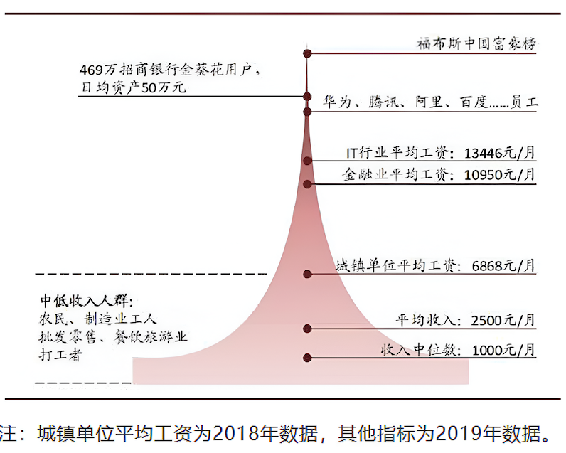
Example 36.1 (Income distribution) The main reason why the median is sometimes preferred over the mean is that the median is more robust to extreme values. A typical example is the income distribution. Higher incomes are rare, but their absolute values are high. Thus, the mean income tends be higher than what the mass of the population would earn. But the median is more robust to extreme values and is closer to the earnings of an “average” person. For example, the average monthly income in China is \(\yen 2,500\) in 2019, but the median is only \(\yen 1,000\).
Theorem 36.1 Let \(X\) be an random variable with mean \(\mu\) , and let \(m\) be a median of \(X\).
- A value of \(c\) that minimizes the mean squared error \(E\left(X-c\right)^{2}\) is \(c=\mu\).
- A value of \(c\) that minimizes the mean absolute error \(E\left|X-c\right|\) is \(c=m\).
Proof.
Minimizing the mean squared error \(E[(X - c)^2]\). Expand the mean squared error: \[E[(X - c)^2] = E[X^2 - 2cX + c^2] = E[X^2] - 2cE[X] + c^2.\] To find the value of \(c\) that minimizes this expression, take the derivative with respect to \(c\) and set it to zero: \[\frac{d}{dc} E[(X - c)^2] = -2E[X] + 2c=0\] This implies \(c=\mu\). We can confirm with second-order condition that \(c = \mu\) is indeed a minimizer.
Minimizing the mean absolute error \(E\left|X-c\right|\). We prove this assuming \(X\) is continuous. \[E|X-c|=\int_{-\infty}^{c}(c-x)f(x)dx+\int_c^{\infty}(x-c)f(x)dx\] Take derivative with respect to \(c\), applying the Leibniz’s rule: \[(c-x)f(x)\frac{d}{dc}c+\int_{-\infty}^c f(x)dx -(x-c)f(x)\frac{d}{dc}c+\int_c^\infty (-f(x))dx=0\] The first-order condition resolves to \[\int_{-\infty}^c f(x) dx = \int_c^{\infty}f(x)dx\] which is exactly the definition of a median.