7 Conditional probability
The probability of A conditioned on B is the updated probability of event A after we learn that event B has occurred. Since events contain information, the occurring of a certain event may change our believes on probabilities of other relevant events. The updated probability of event A after we learn that event B has occurred is the conditional probability of A given B.
Definition 7.1 If \(A\) and \(B\) are events with \(P(B)>0\), then the conditional probability of \(A\) given \(B\) is defined as \[P(A|B)=\frac{P(A\cap B)}{P(B)}.\]
\(P(A|B)\) is the probability of \(A\) occurring given that \(B\) has already occurred. While \(P(A,B)=P(A\cap B)\) is the probability that \(A\) and \(B\) occur simultaneously.
Proposition 7.1 Properties of conditional probability:
\(P(A\cap B)=P(B)P(A|B)=P(A)P(B|A)\)
\(P(A_{1}\cap\cdots\cap A_{n})=P(A_{1})P(A_{2}|A_{1})P(A_{3}|A_{1},A_{2})\cdots P(A_{n}|A_{1}\ldots A_{n-1})\)
Theorem 7.1 (Bayes’ rule) Assume \(P(B)>0\), we have \[P(A|B)=\dfrac{P(B|A)P(A)}{P(B)}\]
The Bayes’ rule is named after Thomas Bayes (18th century) who wanted to know how to infer causes from effects. Human intelligence wants to know the cause given its effects. However, we are only able to observe the effects given the cause. Here is Bayes’ reasoning.
Suppose we have a prior belief about the cause of something we want to learn. We may not be able to learn the true cause directly, but after we observe its effects (the Data), we would update our belief based on the new information we have learned from the data. The updated belief (the posterior) is therefore somewhat closer to the “truth”.
\[\underbrace{P(\text{Belief | Data})}_{\text{Posterier}}= \frac{\overbrace{P(\text{Data | Belief})}^{\text{Likelihood}}\; \overbrace{P(\text{Belief})}^{\text{Prior}} }{P(\text{Data})}\]
Theorem 7.2 (Law of total probability (LOTP)) Let \(B_{1},...,B_{n}\) be a partition of the sample space \(S\) (i.e., the \(B_{i}\) are disjoint events and their union is \(S\)), with \(P(B_{i})>0\) for all \(i\). Then \[P(A)=\sum_{i=1}^{n}P(A|B_{i})P(B_{i}).\]
Theorem 7.3 (Conditional version of LOTP) The law of total probability has an analog conditional on another event \(C\), namely, \[P(A|C) = \sum_{i=1}^{n} P(A|B_i\cap C)P(B_i|C).\]
Example 7.1 Get a random 2-card hand from a standard deck. Find the probability of (a) Both cards are aces given that at least one of them (not necessarily the first one) is an ace; (b) Getting another ace given the first draw is an ace of spade.
Solution. The example shows the subtleness of conditional probabilities. The seemingly indifferent probabilities are in fact different: \[\begin{aligned} P(\textrm{two aces | one ace}) &=\frac{P(\textrm{both aces})}{P(\textrm{one ace})}\\ &=\frac{\binom{4}{2}/\binom{52}{2}}{1-\binom{48}{2}/\binom{52}{2}}\\ &=\frac{1}{33};\\ & \\ P(\textrm{another ace | ace of spade}) &=\frac{P(\textrm{ace of spade \& another ace})}{P(\textrm{ace of spade})}\\ &=\frac{\binom{3}{1}/\binom{52}{2}}{\binom{51}{1}/\binom{52}{2}}\\ &=\frac{1}{17}. \end{aligned}\]
Note that, in the first case, the denominator is interpreted as “at least one ace”; whereas in the second case, it is “ace of space + another card”.
Example 7.2 A disease has a prevalence rate of 10% (i.e., the probability of being infected is 10%). A diagnostic test for the disease has an accuracy of 98%, meaning it correctly identifies infected individuals as positive 98% of the time. Calculate the probability that an individual is infected given that the test result is positive.
Solution. Let \(D\) denote being actually infected by the disease; and \(T\) denote a positive test. The test accuracy means: \(P(T|D)=98\%\). It also means \(P(T|D^{C})=2\%\). We also know that \(P(D)=0.1\). We want to find \(P(D|T)\). Note they are two different conditional probabilities, though we mostly confuse the two in everyday life. The two conditional probabilities are associated with Bayes’ rule: \[\begin{aligned}P(D|T)= & \frac{P(T|D)P(D)}{P(T)}\\ = & \frac{P(T|D)P(D)}{P(T|D)P(D)+P(T|D^{C})P(D^{C})}\\ = & \frac{0.98\times 0.1}{0.98\times 0.1+0.02\times 0.9}\approx 84\%. \end{aligned}\]
Note that how \(P(T|D)\) is far away from \(P(D|T)\)!
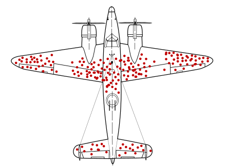
Abraham Wald, the renowned statistician, was hired by the Statistical Research Group (SRG) at Columbia University to figure out how to minimize the damage to bomber aircraft. The data they had comprised aircraft returning from missions with bullet holes on their bodies. If asked which parts of the aircraft should be armored to enhance survivability, the obvious answer seemed to be to armor the damaged parts. However, Wald suggested the exact opposite—to armor the parts that were not damaged. Why? Because the observed damage was conditioned on the aircraft returning. If an aircraft had been damaged on other parts, it likely would not have returned. Thinking conditionally completely changes the answer!
See The Soul of Statistics by Professor Joseph Blitzstein.