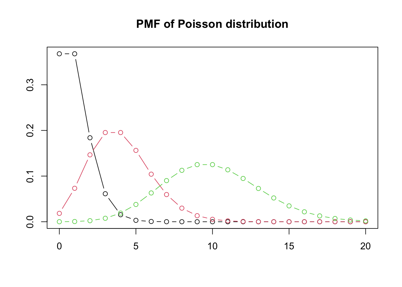
27 Poisson distribution

Now we introduce arguably the most popular discrete distribution—Poisson distribution. Poisson distribution is used to model independent events occurring at a constant mean rate. It is like the Binomial distribution in the sense that they both model the number of occurrence of events, but it is parametrized on the “rate” of the event (how many times an event occurs in a unit of time on average) rather than the total number of events and the probability of each event. It is therefore more practical in real-world modeling since we mostly observe the rate rather than the totality. We introduce the Poisson distribution by showing that it is a limiting case of the Binomial distribution.

Question: Suppose we are studying the distribution of the number of visitors to a certain website. Every day, a million people independently decide whether to visit the site, with probability \(p=2\times10^{-6}\) of visiting. What is the probability of getting \(k\) visitors on a particular day?

We can model the problem with a Binomial distribution. Let \(X\sim \text{Bin}(n,p)\) be the number of visitors, where \(n=10^{6}\) and \(p=2\times10^{-6}\). But it is easy to run into computational difficulties with such a large \(n\) and small \(p\). This is not uncommon, if we want to model the number of emails one receives per day, or the number of phone calls in a service center. In such cases, we could reasonably assume \(n\to\infty\) and \(p\to0\) while \(np=\lambda\) is a constant. We may call \(\lambda\) — the “rate”, as it can be interpreted as the average visitors per day.

Take limit of the Binomial distribution: \[\begin{aligned}P(X=k)= & \lim_{n\to\infty}\binom{n}{k}p^{k}(1-p)^{n-k}\\ = & \lim_{n\to\infty}\binom{n}{k}\left(\frac{\lambda}{n}\right)^{k}\left(1-\frac{\lambda}{n}\right)^{n-k}\\ = & \lim_{n\to\infty}\frac{n!}{(n-k)!k!}\cdot \frac{\lambda^{k}}{n^{k}}\underbrace{\left(1-\frac{\lambda}{n}\right)^{n}}_{\to e^{-\lambda}}\underbrace{\left(1-\frac{\lambda}{n}\right)^{-k}}_{\to1}\\ = & \lim_{n\to\infty}\underbrace{\frac{n!}{n^{k}(n-k)!}}_{\to1}\frac{\lambda^{k}}{k!}e^{-\lambda}\\ = & \frac{\lambda^{k}}{k!}e^{-\lambda}. \end{aligned}\] This is the PMF of the Poisson distribution.

The limiting definition of exponential function

\[e^x = \lim_{n\to\infty}\left(1+\frac{x}{n}\right)^n\]

Definition 27.1 (Poisson distribution) A random variable \(X\) has the Poisson distribution with parameter \(\lambda\) if the PMF of \(X\) is

\[P(X=k)=\frac{e^{-\lambda}\lambda^{k}}{k!},\quad k=0,1,2,\ldots\]

We denote this as \(X\sim\textrm{Pois}(\lambda)\).

We can easily verify this is a valid PMF because \(\sum_{k=0}^{\infty}\frac{\lambda^{k}}{k!}=e^{\lambda}\).

Theorem 27.1 If \(X\sim \text{Bin}(n,p)\) and we let \(n\to\infty\) and \(p\to0\) such that \(\lambda=np\) remains fixed, then the PMF of \(X\) converges to the PMF of \(\text{Pois}(\lambda)\).

The expectation of the Poisson distribution is

\[\begin{aligned}E(X)= & \sum_{k=0}^{\infty}k\cdot\frac{e^{-\lambda}\lambda^{k}}{k!}\\ = & e^{-\lambda}\sum_{k=1}^{\infty}\frac{\lambda^{k}}{(k-1)!}\\ = & \lambda e^{-\lambda}\sum_{k=1}^{\infty}\frac{\lambda^{k-1}}{(k-1)!}\\ = & \lambda e^{-\lambda}e^{\lambda}=\lambda. \end{aligned}\]

Example 27.1 Continued with the website visiting example, there are one million people visiting the site every day, each with probability \(p=2\times10^{-6}\). Give an approximation for the probability of getting at least three visitors on a particular day.

Let \(X\) be the number of visitors. Since \(n\) is large, \(p\) is small, \(np=2\) is fixed, \(X\) is well approximated by \(\text{Pois}(2)\). Therefore, \[\begin{aligned} P(X\geq3)=1-P(X<3) & =1-P(X=0)-P(X=1)-P(X=2)\\ & =1-e^{-2}-2e^{-2}-\frac{2^{2}}{2!}e^{-2}\\ & =1-5e^{-2}\approx0.32.\end{aligned}\]

The Poisson distribution is often used in situations where we are counting the number of successes in a particular region or interval of time, where there are a large number of trials, each with a small probability of success. The Poisson paradigm says in situations like this, we can approximate the number of successes by a Poisson distribution. It is more general than Theorem 27.1, as we relax the assumption of independence and identical events.

Proposition 27.1 (Poisson paradigm) Let \(A_{1},\dots,A_{n}\) be events with \(p_{j}=P(A_{j})\), where \(n\) is large, the \(p_{j}\) are small, and the \(A_{j}\) are independent or weakly dependent. Then \(X=\sum_{j=1}^{n}I(A_{j})\), that is how many of the \(A_{j}\) occur, is approximately distributed as \(\text{Pois}(\lambda)\) with \(\lambda=\sum_{j=1}^{n}p_{j}\).

The Poisson paradigm is also called the law of rare events. The interpretation of “rare” is that the \(p_{j}\) are small, but \(\lambda\) is relatively stable. The number of events that occur may not be exactly Poisson, but the Poisson distribution often gives good approximations. Note that the conditions for the Poisson paradigm to hold are fairly flexible: the \(n\) trials can have different success probabilities, and the trials don’t have to be independent, though they should not be very dependent. So there are a wide variety of situations that can be cast in terms of the Poisson paradigm. This makes the Poisson a very popular model.

Poisson distribution is also used to model the number of events occurring randomly over time with constant rate, such as the number of customers visiting a store, the number of phone calls to a call center, and so on.

Why the random occurrence of events has anything to do with the Poisson distribution? Consider in this way: one can divide the time line into infinitely small intervals (e.g. milliseconds). In each interval, an event either happens or not. The chance that an event occurs in a millisecond is very small. While there are infinitely many trials. So counting events occurring randomly at a fixed average rate over time is mathematically equivalent to counting rare events in many trials.

Definition 27.2 (Poisson process) A sequence of arrivals in continuous time is a Poisson process with rate \(\lambda\) per unit of time if

The number of arrivals in an interval of length \(t\) is distributed \(\text{Pois}(\lambda t)\);
The numbers of arrivals in disjoint time intervals are independent.