Hypothesis testing allows us to test specific hypothesis about a population parameter with the evidence obtained from a sample. The earliest use of statistical hypothesis testing is generally credited to the question of whether male and female births are equally likely (null hypothesis), which was addressed in the 1700s by John Arbuthnot and later by Pierre-Simon Laplace.
Let \(p\) be the population ratio (defined as the ratio of boys to the total number of babies). We hypotheses that \[H_{0}:p=0.5\] This is called the null hypothesis, which is the hypothesis we want to test. If the null hypothesis is false, we have \[H_{1}:p\neq0.5\] This is called the alternative hypothesis. How am I able to test which hypothesis is true? I can answer this question by collecting a small sample. Suppose I have collected a sample of \(50\) babies computed a sample ratio of \(\hat{p}=0.55\). Does it prove or disprove the hypothesis?
Note that the ratio \(\hat{p}\) can be regarded as a sample mean. Let \(X_{i}\) be a random variable that equals \(1\) if the \(i\)-th baby is a boy and \(0\) otherwise. Then, \(\hat{p}=\frac{1}{n}\sum_{i=1}^{n}X_{i}\). The variance of \(\hat{p}\) is given by \[Var(\hat{p})=\frac{1}{n^{2}}\sum_{i=1}^{n}Var(X_{i})=\frac{p(1-p)}{n}\] since \(X_{i}\) is a Bernoulli random variable. By the Central Limit Theorem, we have \[\frac{\hat{p}-p}{\sqrt{\frac{p(1-p)}{n}}}\to N(0,1)\] Suppose \(H_{0}\) is true, then we know the distribution of \(\hat{p}\). In particular, there is 95% chance that \(\hat{p}\) would be in the interval \[p\pm1.96\sqrt{\frac{p(1-p)}{n}}=0.5\pm0.14\] Our observed sample mean \(\hat{p}=0.55\) is not outrageous. It is well within this interval. That means the evidence is not against the null hypothesis. It does not mean \(H_{0}\) is true. But it is reasonable given we have observed a sample mean \(\hat{p}=0.55\).
Suppose we have observed \(\hat{p}=0.65\). This piece of evidence does not seem to be consistent with the null hypothesis. Because if \(H_{0}\) is true, we only have less than 5% chance of observing this sample mean. It is extremely unlikely. Based on this sample, we are more inclined to reject the \(H_{0}\). Rejecting the null hypothesis does not mean it is false, but it means our evidence does not support this hypothesis.
Definitions
Definition 61.1 (Hypothesis testing) A null hypothesis (\(H_0\)) is a statement that there is no relationship or effect between variables. An alternative hypothesis (\(H_1\)) is the opposite of the null hypothesis. Hypothesis testing seeks to find evidence to reject the null.
Definition 61.2 (Power function) In a hypothesis testing about a parameter \(\theta\), let the null hypothesis be \[H_0: \theta = \theta_0\] The power function, \(\pi(\theta)\) is a function that gives the probability of rejecting the null hypothesis when it is true.
An ideal test
An ideal test would be: \(\pi(\theta_0) = 0\), and \(\pi(\theta)=1\). for any \(\theta \leq\theta_0\). That is, the test never makes a mistake. But in reality, a test always involves errors.
Definition 61.3 (Type I/II error) A Type I error is rejecting the \(H_0\) when it is true, whose probability is given by \[\alpha = \pi(\theta_0).\] A Type II error is failing to reject the \(H_0\) when it is false, whose probability is given by \[\beta = 1- \pi(\theta).\]
Type I/II error
Reject \(H_{0}\)
Fail to reject \(H_{0}\)
\(H_{0}\) is true
Type I error
\(\checkmark\)
\(H_{0}\) is false
\(\checkmark\)
Type II error
Definition 61.4 (Significance level) Significance level is the probability of making a Type I error, that is the \(\alpha\).
In a hypothesis testing, we typically want to control the Type I error. That is we want to make sure that when we reject the null, the chance of being wrong is small. Typically, we restrict \(\alpha\) to a very small value, such as \(\alpha = 0.1, 0.05, 0.01\).
Definition 61.5 (p-value) The probability of observing a test statistic as extreme as, or more extreme than, the one calculated from the sample data, assuming \(H_0\) is true. A small \(p\)-value provides strong evidence against\(H_0\).
Definition 61.6 (Decision rule) We reject the null hypothesis (\(H_0\)) under a given significance level (\(\alpha\)) if \(p \leq \alpha\). We say a result is statistically significant, by the standards of the study, when \(p \leq \alpha\).
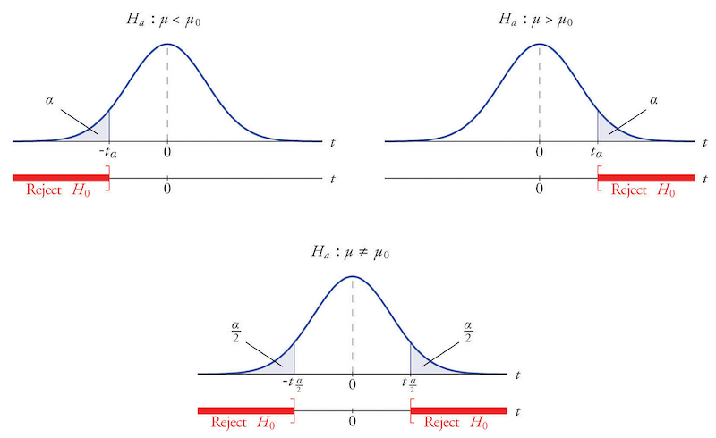
Decision rule of one-sided and two-sided tests
Testing the sample mean
Tom is 185 (cm) tall and he wants to know if he is taller than the average male (\(\mu\)).
We adopt significance level \(\alpha=0.05\). Because \(p<\alpha\), we reject the \(H_0\) and accept \(H_1\). We thus conclude Tom is significantly taller than the average.
Why t-test?
By convention, we would like to use a \(t\)-test. For large samples, \(t\)-statistic converges to standard normal. So it is equivalent to conducting \(z\)-test under CLT. For small samples, \(t\)-test is valid if the sample is drawn from a normal distribution.
Comparing two sample means
Are male students on average do better in exams than female students? (or the other way around)
We adopt significance level \(\alpha=0.05\). Because \(p>\alpha\), we fail to reject the \(H_0\). We thus conclude the average score of male students is not significantly different from females.
Goodness-of-fit test
Purpose: Decide if the values of a categorical variable abide to certain frequencies. For example, are people equally likely to be introverts and extroverts?
Constructing test statistics:\[\chi^2 = \sum_{i=1}^{k} \frac{(O_i - Np_i)^2}{Np_i} \]
where \(O_i\) is the number observations of category \(i\); \(N\) is the total number of observations. The test statistics asymptotically approaches a \(\chi^2(k-1)\) distribution, where \(k\) is the number of categories.
Computing test statistics and p-value:
# load datasetdata <-read.csv("../dataset/survey.csv")# extract heights of malesO1 <-NROW(data[data$Type =='E',])O2 <-NROW(data[data$Type =='I',]) # chi-square test of goodness-of-fitx <-chisq.test(c(O1, O2), p =c(.5, .5))# report resultscat("chisq:", x$statistic, "p-value:", x$p.value)
chisq: 3.188679 p-value: 0.0741499
Making decision:
We’ve got \(p=0.074 >0.05\), so we will not be able to reject the null at 5% significance level. However, the difference is significant at 10% significance level.
Test of independence
Purpose: Decide if two variables are statistically independent. For example, is personality independent of gender?
\[\begin{aligned}
H_0:\ & \text{The two variables are independent} \\
H_1:\ & \text{The two variables are not independent} \\
\end{aligned}\]
Constructing test statistics:
Let \(E_{i,j}\) be the “theoretical frequency” of the value in the \(i\)-th row and \(j\)-th column. If the independent hypothesis is true, then \[E_{i,j} = N p_{i\cdot}p_{\cdot j}\] where \(N\) is the total number of observations and \[p_{i\cdot} = \frac{O_{i\cdot}}{N}, p_{\cdot j} = \frac{O_{\cdot j}}{N}\] is the marginal probability of the row variable and column variable respectively.
The test statistic is \[\chi^2 = \sum_{i=1}^r \sum_{j=1}^c \frac{(O_{i,j}-E_{i,j})^2}{E_{i,j}} \] The test statistic is an asymptotic \(\chi^2(d)\) distribution with a degree of freedom \(d=(r-1)(c-1)\).
Computing test statistics and p-value:
# contingency tablec <-table(data$Gender, data$Type)# chi-square test of independencex <-chisq.test(c)# report resultscat("chisq:", x$statistic, "p-value:", x$p.value)
chisq: 0.3102921 p-value: 0.577501
Making decision:
The fact that \(p=0.58 >0.1\) means we are unable to reject the null even at 10% significance level. Thus we conclude the row variable and column variable are statistically independent.