Definition 19.1 (Binomial distribution) Suppose \(X_{1},X_{2},\dots,X_{n}\) are independent and identical \(\text{Bern}(p)\) distributions. Let \(X\) be the total number of successes of the \(n\) independent trials. That is, \(X=X_{1}+X_{2}+\cdots+X_{n}\). Then \(X\) has the Binomial distribution, \(X\sim \text{Bin}(n,p)\).
The PMF of \(X\) directly follows from the combination theory: \[P(X=k)=\binom{n}{k}p^{k}(1-p)^{n-k}.\]
This is a valid PMF because, by the Binomial theorem, we have \[\sum_{k=0}^{n}\binom{n}{k}p^{k}(1-p)^{n-k}=(p+(1-p))^{n}=1.\]
Binomial distribution and Binomial theorem
You may have noticed the connection between Binomial distribution and Binomial theorem. Consider using the polynomial \(px+q\) to represent the outcome of a single Bernoulli trial, where \(x\) is the indicator for a success. Then \((px+q)^n\) is the outcome for \(n\) independent trials. The coefficient of \(x^k\) gives the probability of there being exactly \(k\) successes.
Theorem 19.1 Let \(X\sim \text{Bin}(n,p)\) and \(Y\sim \text{Bin}(m,p)\) be two independent Binomial random variables. Then \(X+Y\sim \text{Bin}(n+m,p)\).
Proof. By the definition of the Binomial distribution, \(X=\sum_{i=1}^{n}X_{i}\) where \(X_{i}\sim \text{Bern}(p)\); \(Y=\sum_{j=1}^{m}Y_{j}\) where \(Y_{j}\sim \text{Bern}(p)\). Therefore, \[X+Y=\sum_{i=1}^{n}X_{i}+\sum_{j=1}^{m}Y_{j}=\sum_{k=1}^{n+m}Z_{k}\] where \(Z_{k}\sim \text{Bern}(p)\). Since \(X_{i}\) and \(Y_{j}\) are identical Bernoulli random variables, \[Z_k = \begin{cases}X_k,&\text{ for }k=1,\dots,n\\
Y_{k-n}, &\text{ for }k=n+1,\dots,n+m
\end{cases}\] By definition, \(X+Y=\sum_{k=1}^{n+m}Z_{k}\sim \text{Bin}(n+m,p)\).
Coin tossing problem
Example 19.1 In the previous example of tossing two coins, we compute the distribution of \(X\) by counting the equally likely outcomes in an event. We can get the same result by realizing it is a Binomial distribution. \(X\sim\textrm{Bin}(2,1/2)\). Since each coin tossing is an independent Bernoulli trial. The probabilities come directly from the PMF. \[\begin{aligned}
P(X=0) & =\binom{2}{0}\left(\frac{1}{2}\right)^{0}\left(\frac{1}{2}\right)^{2}=\frac{1}{4};\\
P(X=1) & =\binom{2}{1}\left(\frac{1}{2}\right)^{1}\left(\frac{1}{2}\right)^{1}=\frac{1}{2};\\
P(X=2) & =\binom{2}{2}\left(\frac{1}{2}\right)^{2}\left(\frac{1}{2}\right)^{0}=\frac{1}{4}.\end{aligned}\]
Utilizing the Binomial distribution also allows us to generalize the problem. Suppose we are tossing \(n\) coins, we want to find the probability of getting \(k\) heads. It is almost impossible to count all the possible outcomes, but the answer immediately follows from the Binomial PMF.
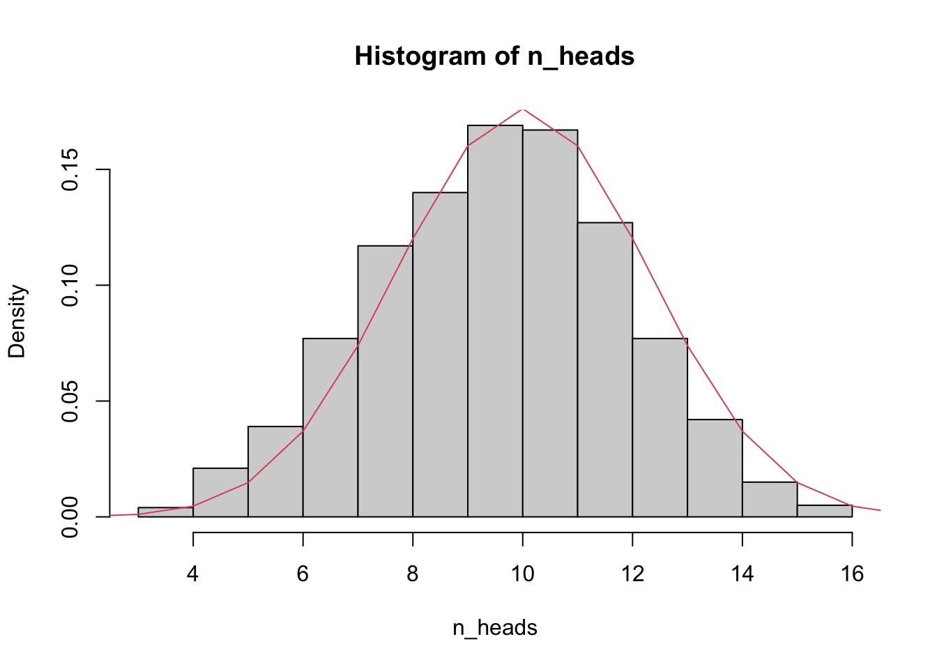
The following code simulates the number of heads if tossing \(N\) coins:
# Number of simulationsk <-1000# Number of coinsn <-20# Store the resultsn_heads <-numeric(k)# Initialize random generatorset.seed(100)# Run simulationsfor (i in1:k) { toss <-sample(c('H','T'), n, replace = T) n_heads[i] <-sum(toss =='H')}# Plot distributionhist(n_heads, probability=TRUE)# Overlay the Binomial PMFcurve(choose(n,x)*0.5^x *0.5^(n-x), from=1, to=n, n=n, col=2, add=T)
Binomial functions in R
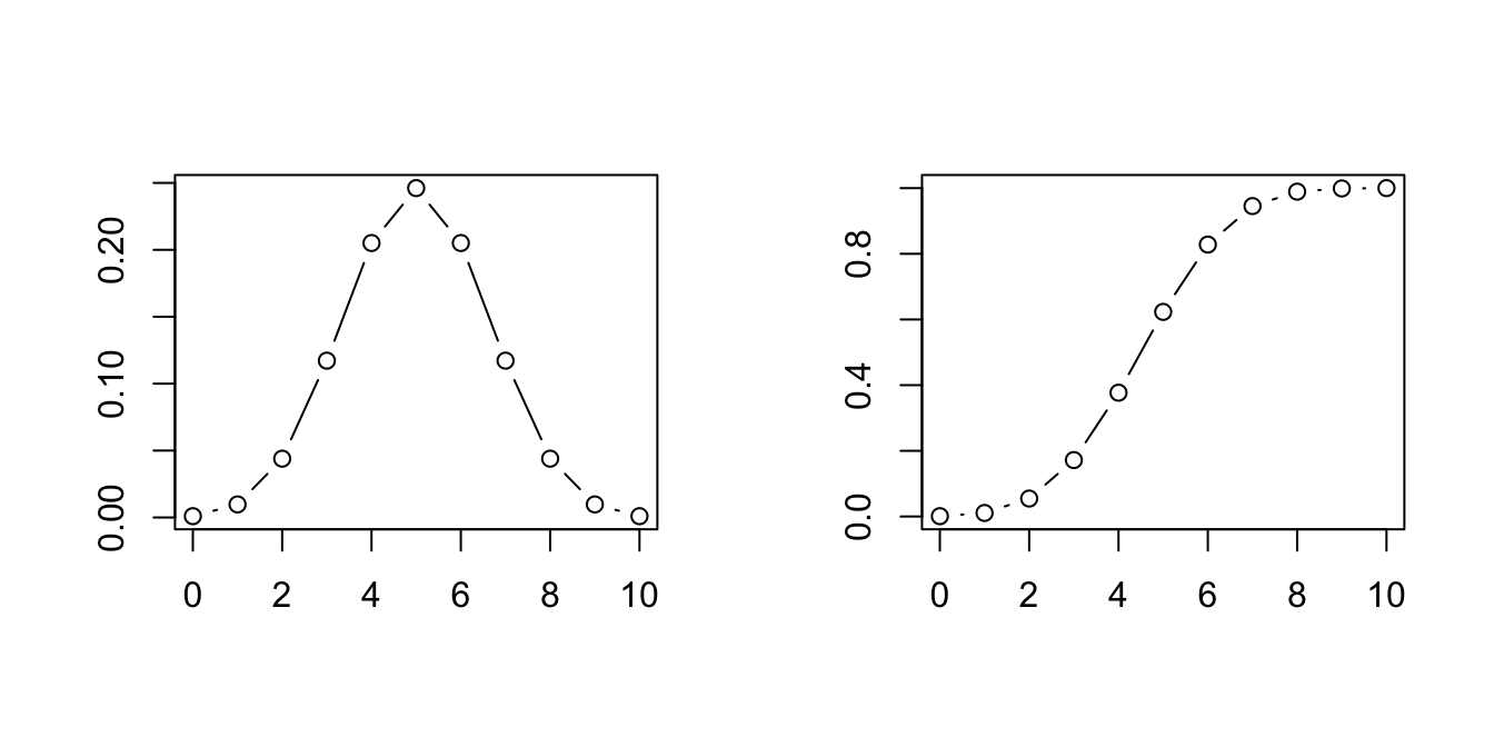
There are built-in functions in R to work with Binomial distributions.
# computes P(X=5) for Bin(10,0.5)p <-dbinom(5, 10, 0.5)par(mfrow=c(1,2))# plot the PMF for Bin(10,0.5)curve(dbinom(x, 10, 0.5), from=0, to=10, n=11, type="b", ann=F)# `pbinom` computes the CDF curve(pbinom(x, 10, 0.5), from=0, to=10, n=11, type="b",ann=F)
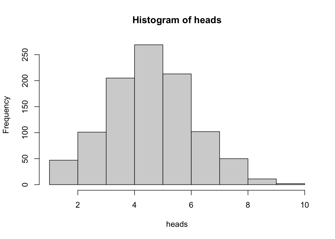
# draw a random value from a given Binomial distribution# this allows us to simulate a random experiment# e.g. the number of heads when flipping 10 fair coinsoutcome <-rbinom(1, 10, 0.5)# Repeat the experiment 1000 timesheads <-rbinom(1000, 10, 0.5)# the histogram will converge to the ideal Binomial distribution# if the experiment is repeated a large number of timeshist(heads)
Exam survival problem
Example 19.2 An exam consists of 20 multiple-choice questions, each with four choices and exactly one correct answer. Suppose a student answers every question by guessing at random. What is the probability that the student passes the exam, defined as answering more than 60% of the questions correctly?
Solution. The probability of correctly answering one question is \(p=1/4\). Let \(N\) be the total number of questions, \(N=20\). Let \(X\) be the number of correctly answered questions, \(X\leq N\). Then \(X\) follows the Binomial distribution \(X \sim B(N, 1/4)\). The probability of passing the exam is therefore \[P(X \geq 12) = 1-P(X\leq 11)=1-\text{CDF}^{\text{Bin}}(11)\approx 0.001.\]
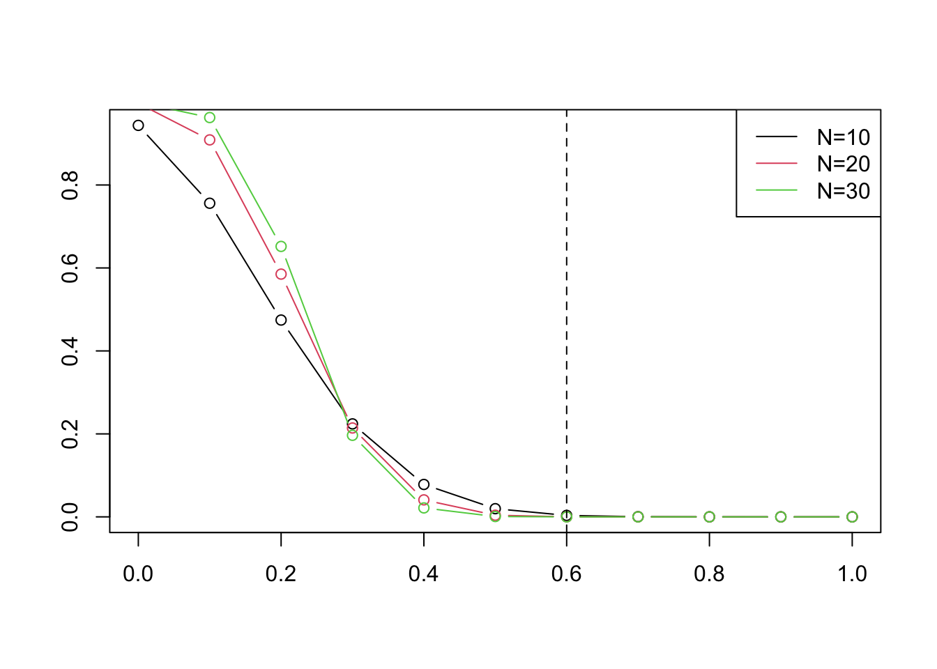
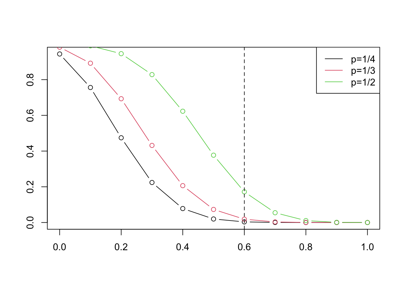
Now we compare the survival probability for different choice of \(N\) and \(p\) :
# Percentage of correct answersx <-seq(0, 1, .1)# Survival probabilities for different Ny1 <-1-pbinom(10*x, 10, .25)y2 <-1-pbinom(20*x, 20, .25)y3 <-1-pbinom(30*x, 30, .25)# Compare the curves for different Nplot(x, y1, type="b", col=1, ann=F)lines(x, y2, type="b", col=2)lines(x, y3, type="b", col=3)# Indicating passing the examabline(v=0.6, lty=2)# Add a legend at the top right corner of the plotlegend("topright", c("N=10", "N=20", "N=30"), lty=1, col=1:3)
# Percentage of correct answersx <-seq(0, 1, .1)# Survival probabilities for different p (number of choices)y1 <-1-pbinom(10*x, 10, .25)y2 <-1-pbinom(10*x, 10, .33)y3 <-1-pbinom(10*x, 10, .5)# Compare the curves for different pplot(x, y1, type="b", col=1, ann=F)lines(x, y2, type="b", col=2)lines(x, y3, type="b", col=3)# Indicating passing the examabline(v=0.6, lty=2)# Add a legend at the top right corner of the plotlegend("topright", c("p=1/4", "p=1/3", "p=1/2"), lty=1,col=1:3)