set.seed(0)

# Repeat experiment: sum of heads tossing ten coins
S1 <- replicate(1000, { sum(sample(0:1, 20, TRUE)) })

hist(S1, prob=TRUE)

# Bell-shaped curve
curve(dnorm(x, mean(S1), sd(S1)), col=2, add=TRUE)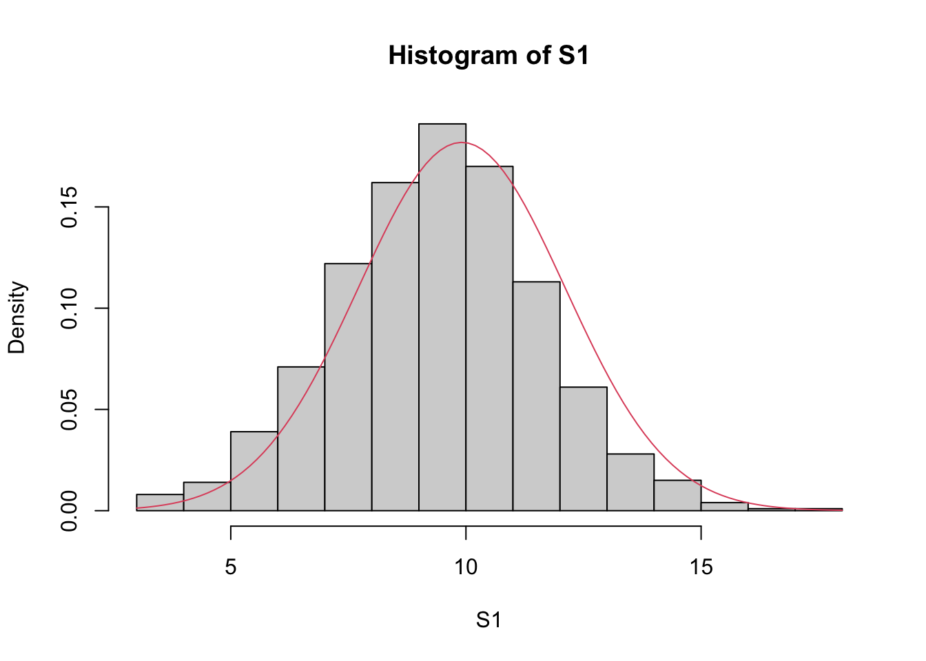
We know the sum of coin heads and the sum of dice points follow a Binomial distribution.
set.seed(0)
# Repeat experiment: sum of heads tossing ten coins
S1 <- replicate(1000, { sum(sample(0:1, 20, TRUE)) })
hist(S1, prob=TRUE)
# Bell-shaped curve
curve(dnorm(x, mean(S1), sd(S1)), col=2, add=TRUE)
The distribution of the sum of dice has a similar shape:
set.seed(0)

# Repeat experiment: sum of rolling ten dice
S2 <- replicate(10000, { sum(sample(1:6, 10, TRUE)) })

hist(S2, prob=TRUE)

# Bell-shaped curve
curve(dnorm(x, mean(S2), sd(S2)), col=2, add=TRUE)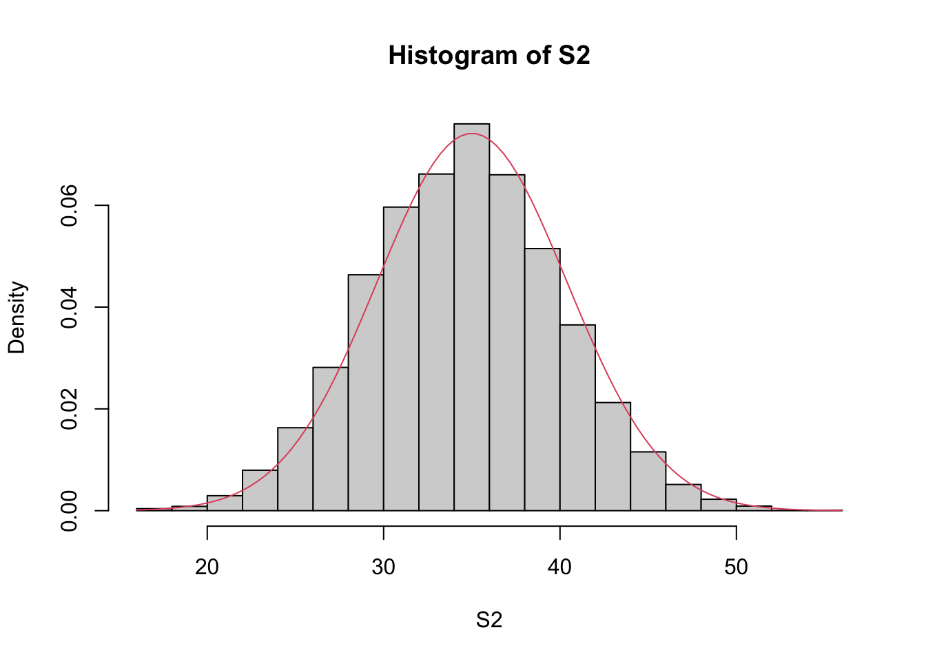
This is not a coincidence. In fact, the sum of random variables from any distribution would reveal a similar shape.
set.seed(0)

# Repeat experiment: sum of ten uniform variables
S3 <- replicate(1000, { sum(runif(10)) })

hist(S3, prob=TRUE)

# Bell-shaped curve
curve(dnorm(x, mean(S3), sd(S3)), col=2, add=TRUE)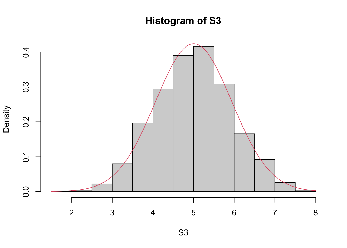
The bell-shaped curve comes from Normal distributions. The distribution of the sum of random variables always converges to Normal distribution.
Let \(X_1, X_2, \dots, X_n\) be a sequence of independent and identical random variables. Let \[S_n = X_1 + X_2 + \dots + X_n\] Then, as \(n\to\infty\), \(S_n\) converges to Normal in distribution. That is \[S_n \to^d \textrm{Normal}.\]