set.seed(0)

# population of uniform distribution
G <- rnorm(10000)

# repeatedly sample from the population and compute sample mean
X_bar <- replicate(1000, mean(sample(G, 100)))

# distribution of the sample mean
hist(X_bar, prob = TRUE)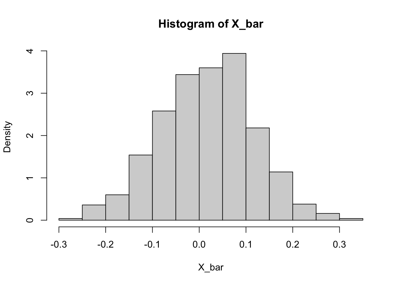
Definition 56.1 (Convergence in distribution) Let \(X_1,X_2,\dots,X_n\) be a sequence of random variables, and let \(F_n\) denote the CDF of \(X_n\). It is said the sequence \(X_1,X_2,...\) converges in distribution \(F\) if \[\lim_{n\to\infty} F_n(x) = F(x),\] for all \(x\) at which F(x) is continuous. The property is denoted as \[ F_n \to_d F. \] \(F\) is called the asymptotic distribution of \(X_n\).
Theorem 56.1 (Central limit theorem) Let \(X_1,X_2,\dots,X_n\) be a random sample of size \(n\) from a distribution with mean \(\mu\) and finite variance \(\sigma^2\). Let \(\bar{X}_n\) be the sample mean. Then, \[\frac{\bar{X}_{n}-\mu}{\sigma/\sqrt{n}} \to_d N(0,1).\]
Note that the CLT can be equivalently expressed as: \[\begin{aligned} \sum_{i=1}^{n} X_i &\to_d N(n\mu, n\sigma^2) \\ \bar{X}_n &\to_d N\left(\mu, \frac{\sigma^2}{n}\right)\\ \frac{\bar{X}_n - \mu}{\sigma} &\to_d N\left(0, \frac{1}{n}\right) \end{aligned}\]
Proof. We will prove the CLT assuming the MGF of the \(X_{i}\) exists, though the theorem holds under much weaker conditions. Without loss of generality let \(\mu=1,\sigma^{2}=1\) (since we standardize it anyway). We show that the MGF of \(\sqrt{n}\bar{X}_{n}=(X_{1}+\cdots+X_{n})/\sqrt{n}\) converges to the MGF of the \(N(0,1)\).
\[\begin{aligned} E(e^{\sqrt{n}\bar{X}_{n}}) & =E(e^{t(X_{1}+\cdots+X_{n})/\sqrt{n}})\\ & =E(e^{tX_{1}/\sqrt{n}})E(e^{tX_{2}/\sqrt{n}})\cdots E(e^{tX_{n}/\sqrt{n}})\\ & =\left[E(e^{tX_{i}/\sqrt{n}})\right]^{n}\qquad\textrm{since }i.i.d\\ & =\left[E\left(1+\frac{tX_{i}}{\sqrt{n}}+\frac{t^{2}X_{i}^{2}}{2n}+o(n^{-1})\right)\right]^{n}\\ & =\left[1+\frac{t}{\sqrt{n}}E(X_{i})+\frac{t^{2}}{2n}E(X_{i}^{2})+o(n^{-1})\right]^{n}\\ & =\left[1+\frac{t^{2}}{2n}+o(n^{-1})\right]^{n}\\ & =\left[1+\frac{t^{2}/2}{n}+o(n^{-1})\right]^{n}\\ & \to e^{t^{2}/2}\qquad\textrm{as }n\to\infty\end{aligned}\]
Therefore, the MGF of \(\sqrt{n}\bar{X}_{n}\) approaches the MGF of the standard normal. Since MGF determines the distribution, the distribution of \(\sqrt{n}\bar{X}_{n}\) also approaches the standard normal distribution.
The distribution of the sample mean \(\bar{X}\) and the distribution of the random variables \(X_i\) are fundamentally different. The former is a theoretical distribution of the averages we would get if we drew repeated samples of size \(n\). What the CLT says is that, regardless the distribution of \(X_i\), the distribution of \(\bar{X}\) always approaches Normal.
set.seed(0)
# population of uniform distribution
G <- rnorm(10000)
# repeatedly sample from the population and compute sample mean
X_bar <- replicate(1000, mean(sample(G, 100)))
# distribution of the sample mean
hist(X_bar, prob = TRUE)
The CLT gives the distribution of the sample mean regardless of the underlying distribution. It allows us to gauge the accuracy of our sample mean as an estimate of the true mean: \[ P\left(\left| \frac{\bar{X}-\mu}{\sigma/\sqrt{n}} \right| \leq 1 \right) = .68 \] \[ P\left(\bar{X}-\sigma^2/\sqrt{n} \leq \mu \leq \bar{X}+\sigma^2/\sqrt{n}\right) = .68 \] Thus, the interval \([\bar{X} - \sigma^2/\sqrt{n}, \bar{X} + \sigma^2/\sqrt{n}]\) contains the true mean 68% of the chance. This is known as confidence intervals that we will come back later. But we need one more theorem to make this actually works.
Theorem 56.2 (Slutsky’s theorem) Let \(X_n\) and \(Y_n\) be sequences of random variables. If \(X_n \to_p c\) and \(Y_n \to_d Y\), then
In practice, the true variance \(\sigma^2\) is unknown. But if we have an estimate from our sample such that \(s^2 \to_p \sigma^2\), the Slutsky’s theorem implies: \[\frac{\bar{X}_{n}-\mu}{s/\sqrt{n}} \to_d N(0,1).\] Thus we can feasibly construct the confidence interval with the sample variance: \([\bar{X} - s^2/\sqrt{n}, \bar{X} + s^2/\sqrt{n}]\).