Definition 24.1 (Negative Binomial distribution) In a sequence of independent Bernoulli trials with success probability \(p\), if \(X\) is the number of failures before the \(r\)-th success, then \(X\) is said to have a Negative Binomial distribution, denoted \(X\sim\textrm{NBin}(r,p)\).
The PMF for Negative Binomial distribution is given by
\[P(X=k)=\binom{k+r-1}{r-1}q^{k}p^{r}.\]
To compute the expectation, let \(X=X_{1}+\cdots+X_{r}\) where \(X_{i}\) is the number of failures between the \((i-1)\)-th success and the \(i\)-th success, \(1\leq i\leq r\). Then \(X_{i}\sim\textrm{Geom}(p)\). By linearity of expectations,
\[E(X)=E(X_{1})+\cdots+E(X_{r})=r\frac{1-p}{p}.\]
Theorem 24.1 Let \(X_1,X_2,...,X_n\) be independent geometric distributions with the same parameter \(p\). Then \[X=X_1+X_2+\cdots+X_n\] is a negative binomial distribution, namely \(X\sim\text{NBin}(n,p)\).
The theorem is straightforward if we interpret \(X_1\) as the number of failures before the 1st success, \(X_2\) as the number of failures between the 1st and 2nd successes, and \(X_n\) be the number of failures between the \((n-1)\)-th and \(n\)-th successes.
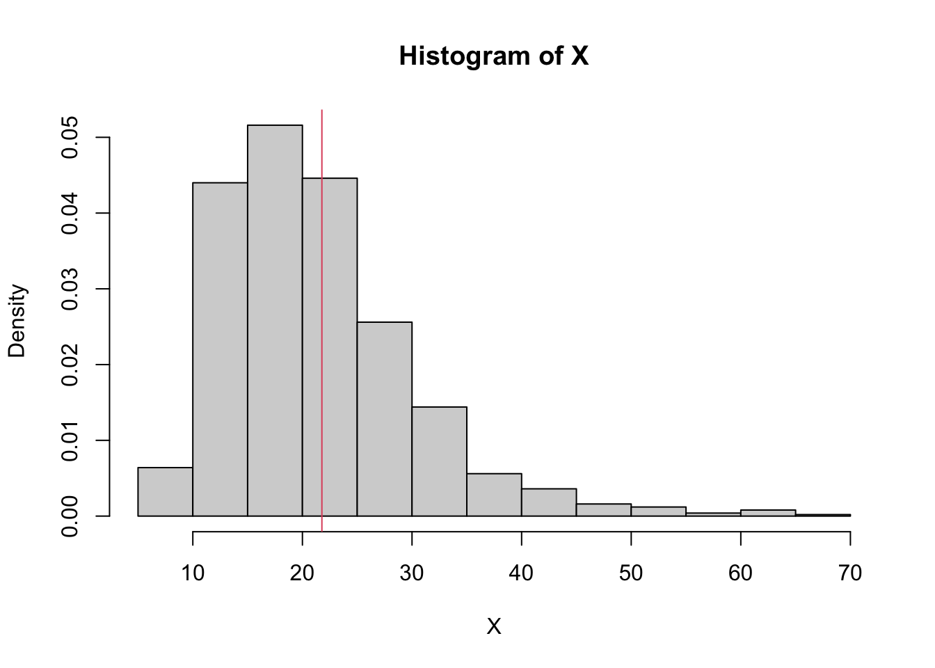
Example 24.1 (Toy collection) There are \(n\) types of toys. Assume each time you buy a toy, it is equally likely to be any of the \(n\) types. What is the expected number of toys you need to buy until you have a complete set?
Solution. Define the following random variables: \[\begin{aligned}T= & T_{1}+T_{2}+\cdots+T_{n}\\
T_{1}= & \textrm{number of toys until 1st new type}\\
T_{2}= & \textrm{additional number of toys until 2nd new type}\\
T_{3}= & \textrm{additional number of toys until 3rd new type}\\
\vdots
\end{aligned}\]
If \(n=5\), \(E(T)\approx11\); if \(n=10\), \(E(T)\approx29\).
# number of simulationsN <-1000# number of toys bought in each simulationX <-numeric(N)# the set of toysToys <-c('🧸','🐢','🐣','🐤','🐼','🤖','🐸','🐷')set.seed(100)# run simulationfor (i in1:N) { C <-c() # the collection of toys bought# repeat until a full set is collectedwhile(TRUE) { t <-sample(Toys, 1, replace=T) C <-c(C, t)if(setequal(C, Toys)) break } X[i] <-length(C)}hist(X, probability = T)abline(v =mean(X), col =2)