60 Confidence intervals
Confidence intervals provide a method of adding more information to an estimator \(\hat{\theta}\) when we wish to estimate an unknown parameter \(\theta\). We can find an interval \((A,B)\) that we think has high probability of containing \(\theta\). The length of such an interval gives us an idea of how closely we can estimate \(\theta\).
Definition 60.1 (Confidence interval) A \(100(1-\alpha)\%\) confidence interval (CI) for \(\theta\) is an interval \([a, b]\) such that the probability that the interval contains the true \(\theta\) is \((1-\alpha)\).
Confidence intervals are reported to indicate the degree of precision of our estimates. The narrower the confidence interval, the more precise the estimate.
We seek an interval which includes the true value with reasonably high probability. Standard choices are \(\alpha=0.05\), corresponding to 95% confidence intervals.
Example 60.1 (CI of a Bernoulli parameter) Suppose we want to know if a coin is fair or not by counting the number of Heads out of \(n\) tosses. Let \(X_{i}\) be a Bernoulli random variable that equals \(1\) if the \(i\)-th toss is Head (with probability \(p\)) and \(0\) otherwise. Given a sample of size \(n\): \(\{X_1, ..., X_n\}\). We want to estimate the parameter \(p\).
In Example 58.1, we find the MLE: \(\hat p = \bar{X}\). But we do not know how close this estimator is to the true value. Suppose we calculated \(\hat p=0.55\) from a sample of 50. Does that mean the coin is unfair? Or is it just a measurement error due to the small sample size?
To get an idea of how precise our estimator is, we would like to construct an interval around \(\hat p\) which contains the true \(p\) with high probability. Since, \[\begin{aligned} E(\hat p) &= E(\bar{X}) = p, \\ Var(\hat p) &= Var(\bar{X}) = \frac{p(1-p)}{n}. \end{aligned}\] By the CLT and the Slutsky’s theorem, \[Z = \frac{\hat p - p}{\sqrt{\frac{\hat p(1-\hat p)}{n}}} \to_d N(0,1).\] Since, \(P(|Z|<1.96) = .95\). The 95% confidence interval is given by \[\hat p \pm 1.96\sqrt{\frac{\hat p(1-\hat p)}{n}}.\]
For \(n=50\), \(\hat p=0.55\), the CI is \([0.41, 0.69]\). That is, the true ratio can be any value between this range. We cannot exclude the possibility of a fair coin.
CI of sample mean
Suppose we want to construct a \((1-\alpha)\) CI of the sample mean \(\bar X_n\). Assume the population mean and variance are \(\mu\) and \(\sigma^2\). Also assume the sample size \(n\) is large enough to invoke the CLT (usually \(n > 30\)). We thus have \[\begin{aligned} \frac{\bar{X}_{n}-\mu}{\sigma/\sqrt{n}} & \sim N(0,1)\end{aligned}\]
Let’s find the interval \([-z,z]\) such that \[P\left(\frac{|\bar{X}_{n}-\mu|}{\sigma/\sqrt{n}}< z\right)=\Phi(z)-\Phi(-z)=1-\alpha\] We thus have: \(z= \Phi^{-1}(1-\alpha/2)\). We denote this value as \(z_{\alpha/2}\).
With a little rearrangement, we have \[P\left(\bar{X}_{n} - z_{\alpha/2}\frac{\sigma}{\sqrt{n}}\leq \mu \leq\bar{X}_{n} + z_{\alpha/2}\frac{\sigma}{\sqrt{n}}\right)=1-\alpha\]
In practice, because we do not know the true \(\sigma^2\), we thus replace it with the sample variance \(s^2\). Theorem 56.2 ensures the result still holds if the sample size is reasonably large.
Theorem 60.1 (Confidence interval of sample mean) The \(100(1-\alpha)\%\) confidence interval for the sample mean \(\bar{X}_{n}\) is \[\left[ \bar{X}_{n}- z_{\alpha/2}\frac{s}{\sqrt{n}}, \bar{X}_{n}+ z_{\alpha/2}\frac{s}{\sqrt{n}} \right],\] where \(s^2\) is the sample variance. \(z_{\alpha/2}\) is called the critical value given the confidence level. The expression \(z_{\alpha/2}\frac{s}{\sqrt{n}}\) is known as the margin of error.
Some commonly used confidence levels
- 90% CI: \(\alpha=0.10\), \(z_{0.050}=1.65\)
- 95% CI: \(\alpha=0.05\), \(z_{0.025}=1.96\)
- 99% CI: \(\alpha=0.01\), \(z_{0.005}=2.58\)
Interpretation of CIs
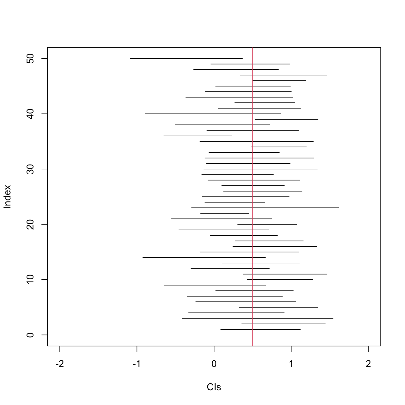
A 95% CI means: 95% of the intervals constructed will cover the true population mean \(\mu\). After taking the sample and an interval is constructed, the constructed interval either covers \(\mu\) or it doesn’t. But if we were able to take many such samples and reconstruct the interval many times, 95% of the intervals will contain the true mean.
Common misconceptions
Suppose we have a 95% confidence interval \([2.7,3.7]\). Which of the following statements is true?
1. We are 95% confident that the sample mean is between 2.7 and 3.7.
False. The CI definitely contains the sample mean \(\bar{X}\).
2. 95% of the population observations are in 2.7 to 3.7.
False. The CI is about covering the population mean, not for covering 95% of the entire population.
3. The true mean falls in the interval [2.7, 3.7] with probability 95%.
False. The true mean \(\mu\) is a fixed number, not a random one that happens with a probability.
4. If a new random sample is taken, we are 95% confident that the new sample mean will be between 2.7 and 3.7.
False. The confidence interval is for covering the population mean, not for covering the mean of another sample.
5. This confidence interval is not valid if the population or sample is not normally distributed.
False. The construction of the CI only uses the normality of the sampling distribution of the sample mean (by the CLT). Neither the population nor the sample is required to be normally distributed.
Applications
Do male students do better in exams than female students? (or the other way around?) Comparing the means are not enough, because there are errors in the estimates.
Let \(\bar{X}_1\) and \(\bar{X}_2\) be the average scores of male and female students respectively. By the CLT, \[\bar{X}_1 \to_d N\left( \mu_1, \frac{\sigma_1^2}{n_1} \right)\] \[\bar{X}_2 \to_d N\left( \mu_2, \frac{\sigma_2^2}{n_2} \right)\]
The difference in sample means also follows a normal distribution: \[\bar{X}_1 - \bar{X}_2 \sim N\left( \mu_1-\mu_2, \frac{\sigma_1^2}{n_1} + \frac{\sigma_2^2}{n_2}\right)\]
We construct a confidence interval over \(\bar{X}_1 - \bar{X}_2\) and check if it contains \(0\).
# load dataset
data <- read.csv("../dataset/survey.csv")

# math scores of introverts and extroverts
x <- data[data$Gender == 'F', 'Score']
y <- data[data$Gender == 'M', 'Score']

d <- mean(x) - mean(y)
s <- sqrt(sd(x)/length(x) + sd(y)/length(y))

ci <- c(d-1.96*s, d+1.96*s)

# CI contains 0, meaning there is no significant difference
cat("Diff:", d, "CI:", ci)
Diff: 1.077273 CI: -0.474347 2.628892The fact that the confidence interval contains \(0\) means that there is no statistical difference between the two means. The algebraic difference is due to errors in the estimation (maybe because of small samples).