41  Moments and MGF

Definition 41.1 (Moment) Let \(X\) be a random variable with mean \(\mu\) and variance \(\sigma^{2}\) . For any positive integer \(n\), the \(n\)-th moment of \(X\) is \(E(X^{n})\), the \(n\)-th central moment is \(E(X-\mu)^{n}\), and the \(n\)-th standardized moment is \(E\left(\frac{X-\mu}{\sigma}\right)^{n}\).

In accordance with this terminology, \(E(X)\) is the first moment of \(X\), \(Var(X)\) is the second central moment of \(X\). It is natural to ask if there are higher order moments. The answer is yes.

Definition 41.2 (Skewness) Let \(X\) be a random variable with mean \(\mu\), standard deviation \(\sigma\), and finite third moment. The skewness of \(X\) is defined as \[\textrm{Skew}(X)=E\left[\left(\frac{X-\mu}{\sigma}\right)^{3}\right].\]

Definition 41.3 (Kurtosis) The Kurtosis of \(X\) is defined as \[\textrm{Kurt}(X)=\left[\left(\frac{X-\mu}{\sigma}\right)^{4}\right].\]

Skewness is the measure of the lopsidedness of the distribution; any symmetric distribution will have a third central moment, if defined, of zero. A distribution that is skewed to the left (the tail of the distribution is longer on the left) will have a negative skewness. A distribution that is skewed to the right (the tail of the distribution is longer on the right), will have a positive skewness.

Kurtosis is a measure of the heaviness of the tail of the distribution. If a distribution has heavy tails, the kurtosis will be high; conversely, light-tailed distributions have low kurtosis.

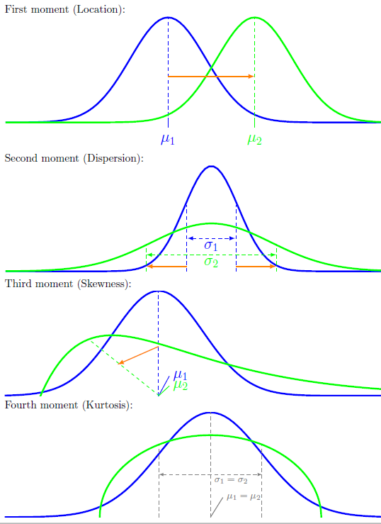
We see that moments give information about the shape of a distribution. Different orders of moments captures different aspects of the distribution. As higher and higher moments are calculated, they reveal more and more aspects of the distribution. Loosely speaking, it is somewhat like the Taylor theorem in the probability theory. We can approximate a distribution by “expectation of polynomials”: \(E(X),E(X^{2}),E(X^{3}),\ldots\)

Definition 41.4 (Moment generating function) Let \(X\) be a random variable. For each real number \(t\), define the moment generating function (MGF) as \[M_{X}(t)=E\left(e^{tX}\right).\]

To see why it is “generating” moments, take the Taylor expansion of the exponential function: \[e^{tX}=1+tX+\frac{t^{2}X^{2}}{2!}+\frac{t^{3}X^{3}}{3!}+\cdots\] Hence, \[M_{X}(t)=E\left(e^{tX}\right)=1+E(X)t+E(X^{2})\frac{t^{2}}{2!}+\cdots\]

A natural question at this point is: What is the interpretation of \(t\)? The answer is that \(t\) has no interpretation in particular; it’s just a bookkeeping device that we introduce in order to encode the sequence of moments in a differentiable function.

Theorem 41.1 Let \(M_{X}(t)\) be the MGF of \(X\). Then the \(n\)-th moment of \(X\) is given by \(E(X^{n})=M_{X}^{(n)}(0)\), where \(M_{X}^{(n)}\) denotes the \(n\)-th derivative of the MGF.

Theorem 41.2 If the MGFs of two random variables \(X_1\) and \(X_2\) are finite and identical for all values of \(t\) in an open interval around the point \(t = 0\), then the probability distributions of \(X_1\) and \(X_2\) must be identical.

Theorem 41.3 If \(X\) and \(Y\) are independent, then the MGF of \(X+Y\) is the product of the individual MGFs: \[M_{X+Y}(t)=M_{X}(t)M_{Y}(t).\]

Example 41.1 For \(X\sim \textrm{Bern}(p)\), \(e^{tX}\) takes on the value \(e^{t}\) with probability \(p\) and the value \(1\) with probability \(q\), so \(M(t)=E\left(e^{tX}\right)=pe^{t}+q\). Since this is finite for all values of \(t\), the MGF is defined on the entire real line.

Example 41.2 The MGF of a \(\textrm{Bin}(n,p)\) random variable is \(M(t)=(pe^{t}+q)^{n}\), since it is the product of \(n\) independent Bernoulli MGFs.