Imagine you are a shop owner that waits for your next customer. The customers arrive randomly. What interests us is the waiting time until the next customer arrives.
Let \(X\) represent the waiting time. Since the customers arrives randomly, the likelihood of it coming in the next moment is the same whether you’ve been waiting for one minute or ten minutes. In other words, the probability of waiting another \(t\) minutes is the same no matter how long you’ve already waited. Therefore, \[P(X\geq s+t\mid X\geq s)=P(X\geq t),\quad\forall s,t\geq0.\] The conditional probability can be rewritten using the definition of conditional probabilities: \[P(X\geq s+t\mid X\geq s)=\frac{P(X\geq s+t)}{P(X\geq s)}.\] Thus, the memoryless property implies: \[\frac{P(X\geq s+t)}{P(X\geq s)}=P(X\geq t).\] Let the survival function \(S(x)\) represent \(P(X\geq x)\) . Substituting \(S(x)\) into the equation gives: \[\frac{S(s+t)}{S(s)}=S(t).\] This reminds us of the exponential function. In fact, the only continuous and non-negative solution to this equation is: \[S(x)=e^{-\lambda x},\quad\lambda>0,\] where \(\lambda\) is a positive constant. This solution represents the probability that the waiting time exceeds \(x\) , and \(\lambda\) determines how quickly the probability decreases over time.
The CDF of \(X\) is exactly the opposite of \(S(x)\): \[F(x)=1-S(x)=1-e^{-\lambda x}.\] Take derivative to get the PDF: \[f(x)=F'(x)=\lambda e^{-\lambda x}.\]
Definition 50.1 (Exponential distribution) A random variable \(X\) is said to have the Exponential distribution with parameter \(\lambda\) if its PDF is \[f(x)=\lambda e^{-\lambda x},\qquad x>0.\]
We denote this as \(X\sim\textrm{Exp}(\lambda).\)\(\lambda\) is interpreted as the “rate”, i.e. number of events per unit of time.
To compute the expectation and variance, we first standardize the exponential distribution. Let \(Y=\lambda X\), then \(Y\sim\textrm{Exp}(1)\), because \[P(Y\leq y)=P(X\leq y/\lambda)=1-e^{-y}.\] It follows that, \[\begin{aligned}
E(Y) & =\int_{0}^{\infty}ye^{-y}dy=\left[-ye^{-y}\right]_{0}^{\infty}+\int_{0}^{\infty}e^{-y}dy=1;\\
Var(Y) & =E(Y^{2})-(EY)^{2}=\int_{0}^{\infty}y^{2}e^{-y}dy-1=1.\end{aligned}\] For \(X=Y/\lambda\), we have \(E(X)=\frac{1}{\lambda}\), \(Var(X)=\frac{1}{\lambda^{2}}\).
Theorem 50.1 (Memoryless property) If \(X\) has the exponential distribution with parameter \(\lambda\), and let \(t>0\), \(h>0\), then \[P(X\geq t+h|X\geq t)=P(X\geq h).\]
Proof. For \(t>0\) we have \[P(X\geq t)=\int_{t}^{\infty}\lambda e^{-\lambda x}dx=e^{-\lambda t}.\] Hence for each \(t>0\) and each \(h>0\), \[P(X\geq t+h|X\geq t)=\frac{P(X\geq t+h)}{P(X\geq t)}=\frac{e^{-\lambda(t+h)}}{e^{-\lambda t}}=e^{-\lambda h}=P(X\geq h).\]
The memoryless property is a very special property of the Exponential distribution. In fact, the Exponential is the only memoryless continuous distribution (with support \((0,\infty)\)); and Geometric distribution is the only memoryless discrete distribution (with support \(0,1,\dots\)).
Theorem 50.2 (Poisson-Exponential connection) Let \(T\) be the time between two consecutive events in Poisson process \(\text{Pois}(\lambda t)\). Then \(T\) follows Exponential distribution \(T\sim\text{Exp}(\lambda)\).
Proof. The waiting time \(T>t\) is equivalent to no event occurred during period \(t\). Therefore, \[P(T>t)=P(N_{t}=0)=e^{-\lambda t}\frac{(\lambda t)^{0}}{0!}=e^{-\lambda t}\] where \(N_{t}\) is the number of events occurred in \([0,t]\), which follows a Poisson distribution. The CDF of \(T\) is
\[F(t)=1-P(T>t)=1-e^{-\lambda t}\]
The PDF of \(T\) is \[f(t)=F'(t)=\lambda e^{-\lambda t}\] This indicates \(T\sim \text{Exp}(\lambda)\).
Example 50.1 (Bus arrivals) We try to model the waiting time at a bus station. Suppose the bus arrives at random time but on average there will be one bus per 10 minutes. You arrive at the bus stop at a random time, not knowing how long ago the previous bus came. What is the distribution of your waiting time for the next bus? What is the mean waiting time? What is the median waiting time?
Solution. The bus arrivals in a period of time is best modeled by a Poisson distribution. Let \(X\) be the waiting time and we know it is an Exponential distribution. Since \(E(X)=1/\lambda=10\), \(X\sim\textrm{Exp}(1/10)\). Thus, The average waiting time is always 10 minutes.
The CDF of \(X\) is \(F(x)=1-e^{-\lambda x}\). The median \(m\) satisfies \(F(m) = 1/2\). Thus, \(m= \log(2)/\lambda \approx 6.9\) minutes. So the typical waiting experienced by most passengers is less than 10 minutes.
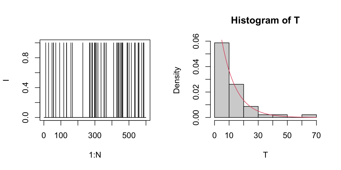
# Simulate random arrivals and inter-arrival timeN <-600# total simulation timep <- .1# prob of occurrence per unit timeset.seed(0) # I[t] = 1 if an event occurs in time t I <-1* (runif(N) < p) par(mfrow=c(1,2))# plot the random occurrenceplot(1:N, I, type ="h")# inter-arrival timeT <-diff( (1:N)[I==1] )# distribution if waiting time hist(T, prob=TRUE)# Overlay the exponential functioncurve(exp(-x/10)/10, col =2, add =TRUE)